ATM and MPLS: the networks behind the classic network calculus examples
Network calculus grew up in the 1990s, when the networks that promised quality of service were ATM and, a little later, IP with IntServ, DiffServ and MPLS. That is why its textbooks speak of cells, leaky buckets, virtual circuits and label-switched paths. This post explains those networks just enough to read the classic examples, and shows that the same ideas reappear in TSN and DetNet.
1. Why these two networks
Both networks fix the path before the data flows, check the traffic at the entry, and switch on a short label instead of a full address. Each of those choices maps onto a network calculus object:
| Network choice | Network calculus object |
|---|---|
| A traffic contract checked at the entry | An arrival curve, enforced by a policer or a greedy shaper |
| A fixed path through known switches | A concatenation of service curves |
| Admission control before the circuit or path is set up | A check that the delay and backlog bounds still hold |
| Classes sharing a queue | Aggregate multiplexing and residual service |
The standard textbook by Le Boudec and Thiran uses the ATM generic cell rate algorithm among its first examples of arrival curves, and its second chapter applies the theory to IntServ and DiffServ [5]. The deterministic networking post summarises IntServ and DiffServ.
2. ATM in brief
Asynchronous Transfer Mode is a cell-switching standard of the ITU-T and ANSI, designed in the late 1980s for the broadband ISDN. It aimed to carry voice, video and data on one network [1]. Its main features:
- Fixed cells of 53 bytes: a 5-byte header and a 48-byte payload. Small, equal cells keep queuing delay and delay variation low. At 155 Mbit/s a 1500-byte packet occupies the link for about 77 µs, and on a 1.544 Mbit/s T1 line for about 7.8 ms, far too long for voice to wait behind several of them. The 48-byte payload was a political compromise between the 64 bytes proposed by the United States and the 32 bytes proposed by Europe [1].
- Connection-oriented. A virtual circuit is set up before any cell is sent. It is either permanent, configured by the operator, or switched, set up by signalling for each call. When a switched circuit is requested, the network performs call admission control: it checks that a route exists with enough resources for the requested traffic [1].
- Label swapping. Each cell carries a virtual path identifier (VPI) and a virtual channel identifier (VCI). Every switch replaces them with the values for the next link. The values change from hop to hop, but the circuit, and so the path, stays the same for every cell [1].
- Adaptation layers (AAL1, AAL2, AAL5, …) adapt services such as circuit emulation, variable-rate media and data to the cell stream [1].
Service categories
When a circuit is set up, each switch on it learns the traffic contract of the connection [1]:
| Category | Contract | Typical use |
|---|---|---|
| CBR, constant bit rate | Peak cell rate (PCR) | Circuit emulation, voice |
| VBR, variable bit rate (real-time and non-real-time) | Sustainable cell rate (SCR), PCR, maximum burst size (MBS) | Compressed video, bursty data |
| ABR, available bit rate | A guaranteed minimum rate | Data that adapts to feedback |
| UBR, unspecified bit rate | None: whatever capacity remains | Best effort |
Most categories also define a cell delay variation tolerance (CDVT). It states how much cells may bunch together after crossing earlier equipment [1].
3. The ATM contract as an arrival curve
At the user–network interface (UNI), and between networks, ATM polices each circuit against its contract. The reference algorithm is the Generic Cell Rate Algorithm, GCRA(, ), where is the nominal spacing between cells and the tolerance [1][3].
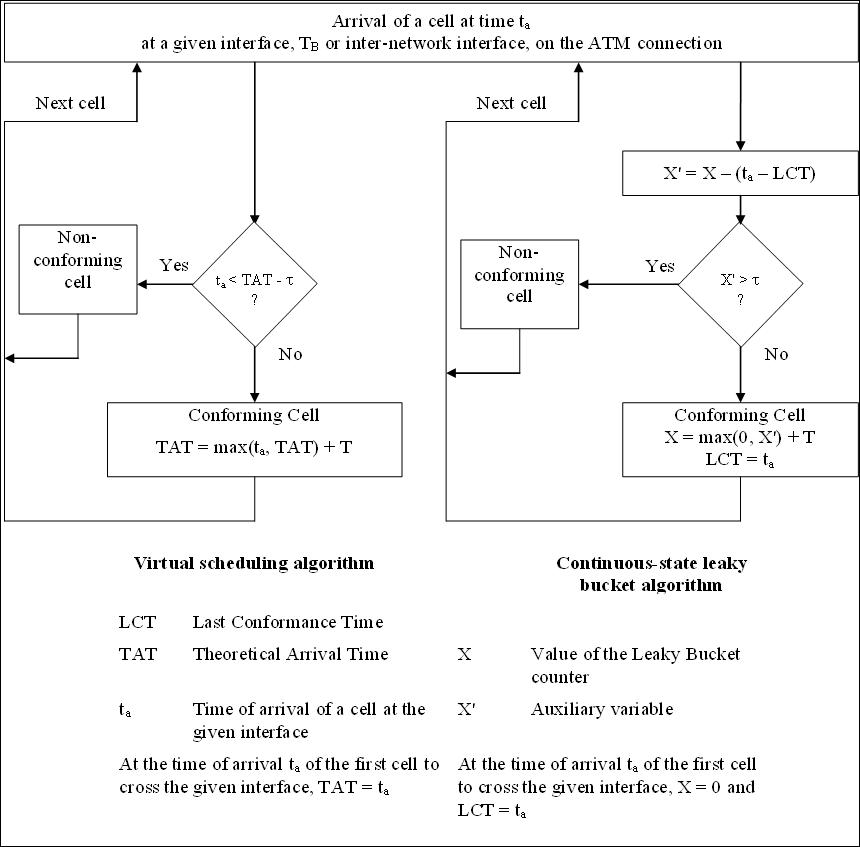

The virtual scheduling form reads almost like a definition of an arrival curve. A cell is conforming if it does not arrive more than before its theoretical time, and each conforming cell pushes the theoretical time further. A cell stream is GCRA(, )-conforming if and only if it has the staircase arrival curve
which is upper-bounded by the token bucket with cells per second and cells [5]. This is the staircase of the arrival curves post, where the tolerance plays the role of the jitter .
VBR: two buckets, one concave curve
A VBR connection is policed by two GCRAs at once, one on the peak rate and one on the sustainable rate [1][3]:
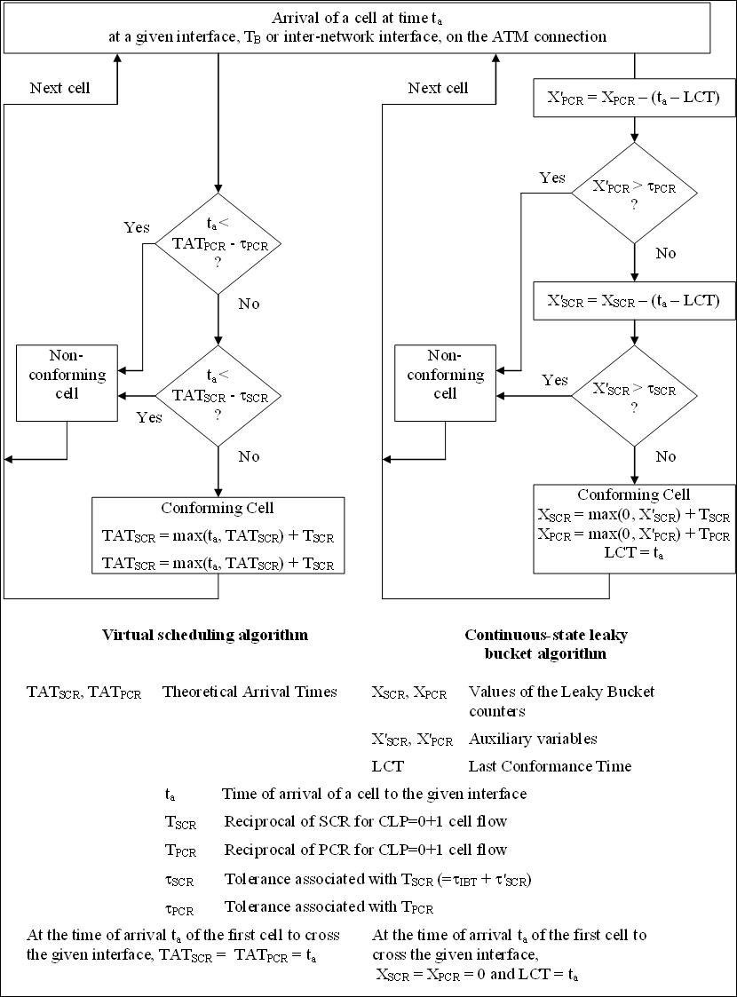

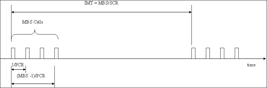

A stream that passes both tests has the minimum of the two curves as its arrival curve. Write the burst tolerance of the sustainable-rate test as and ignore the CDVT. The arrival curve, in cells, is then
This concave, two-piece curve has the same shape as the IntServ traffic specification and as the curves used for TSN streams. Only the units changed.
Worked example
Take a VBR circuit with cells/s, cells/s and cells. Then ms, so
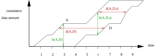
Suppose each switch guarantees the circuit a rate-latency service with cells/s (about 8.5 Mbit/s of cells) and ms. The two pieces of meet at ms. The largest horizontal distance between and lies at that kink, which gives the delay bound
with , , and . Using only the token bucket would give ms, so the peak rate saves a quarter of a millisecond. The backlog bound is the largest vertical distance. It occurs at : cells, about 2.9 kB. The fundamental bounds post derives both distances in general.

Policing and shaping in practice
A cell that breaks the contract is either dropped or tagged by setting its cell loss priority (CLP) bit, so that a congested switch drops it first [1]. Dropping single cells wastes capacity, because one lost cell ruins a whole AAL5 packet. Switches therefore use early or partial packet discard to drop whole packets [1]. On the sending side, the network interface shapes the cell stream so that it conforms before it reaches the UNI [1]. In network calculus this is the greedy shaper: shaping a flow to its own arrival curve does not increase its worst-case delay bound.
4. MPLS in brief
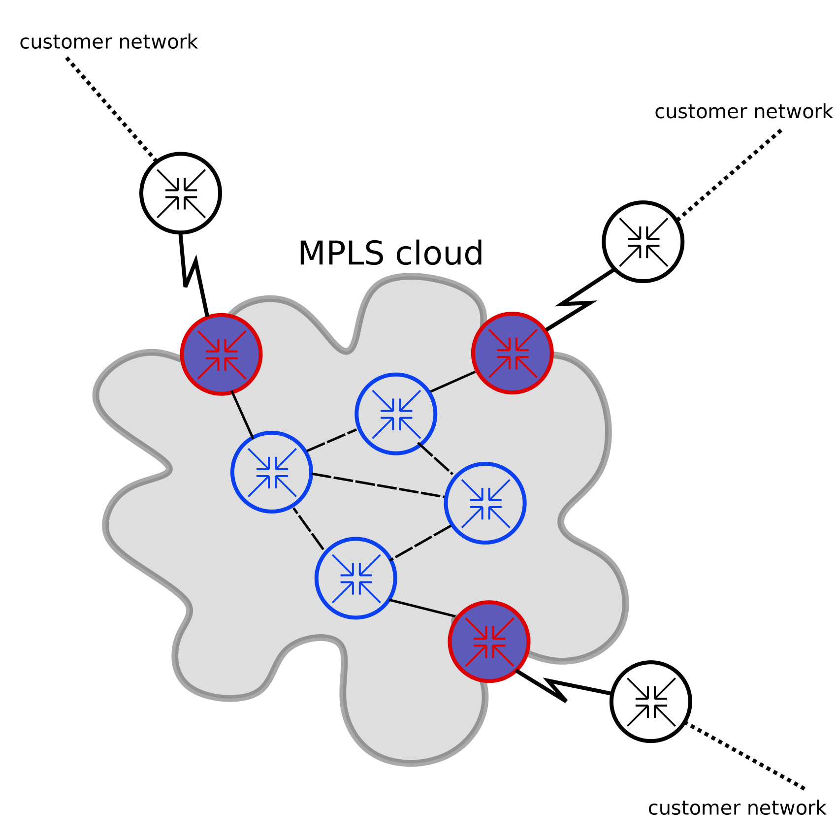

Multiprotocol Label Switching, standardised by the IETF in RFC 3031, forwards packets on a short label instead of the destination address [2][4]. It grew out of IP switching over ATM and Cisco's tag switching, and the IETF working group was formed in 1997 [2]. MPLS kept what made ATM attractive, connection-oriented paths and traffic engineering, while dropping cells and ATM signalling. Modern links are fast enough that a full 1500-byte packet no longer causes a significant queuing delay: about 1.2 µs at 10 Gbit/s [1][2].
- The ingress label edge router (LER) assigns each packet to a forwarding equivalence class (FEC) and pushes a label [2].
- Each label switch router (LSR) looks up the label, swaps it, and forwards the packet [2].
- The egress LER pops the label and forwards plain IP [2].
- The sequence of labels forms a label-switched path (LSP), much like a permanent virtual circuit in ATM, but independent of any layer-2 technology [2].
- Labels are distributed by LDP, or by RSVP-TE when a path with a bandwidth reservation is needed [2].
- Each label stack entry has a 20-bit label, a 3-bit traffic class (TC) for QoS, a bottom-of-stack bit and a TTL (Figure 2). Labels can be stacked, which is how VPNs and tunnels nest [2].
MPLS is now used mostly for traffic engineering, DiffServ quality of service and VPNs [2].
5. MPLS in network calculus terms
An LSP is a fixed path. Its end-to-end service is the min-plus convolution of the per-hop service curves. "Pay bursts only once" applies to it directly, as in the concatenation post.


A TC class is an aggregate. In an MPLS core, packets are queued by traffic class, not by LSP, so a flow shares its queue with every other flow of its class. This is the setting of aggregate multiplexing. It is also where a classic warning comes from. For a network of FIFO aggregates, as in a DiffServ or MPLS core, the known general delay bound holds only if utilisation stays below roughly , where is the longest path in hops [6]. Per-flow reservation at the edge, as with RSVP-TE, keeps each aggregate within its budget.
DetNet reuses MPLS. One of the two DetNet data planes is MPLS. Labels identify the DetNet flow, and a control word carries the sequence number used for packet replication and elimination [7]. The IETF DetNet post describes the architecture.
6. Then and now
| ATM | MPLS | TSN | DetNet | |
|---|---|---|---|---|
| Unit | 53-byte cell | Packet with a label stack | Ethernet frame | IP or MPLS packet |
| Path | Virtual circuit (VPI/VCI) | Label-switched path | Stream on a configured path | DetNet flow on an explicit route |
| Traffic contract | PCR, SCR, MBS, CDVT | Reserved bandwidth (RSVP-TE) or class | Traffic specification (token bucket) | Traffic specification |
| Entry check | GCRA policing at the UNI | Policing at the ingress LER | PSFP | Ingress policing and shaping |
| Admission control | Call admission control (PNNI) | Traffic-engineering reservation | SRP, RAP or CNC | Controller plane |
| Network calculus view | Staircase or two-piece arrival curve | Concatenation and aggregates | Arrival curves, shaper service curves | Same, across L2 and L3 segments |
The vocabulary changed, but the structure did not: a contract at the edge, a known path, and a check before admission. This is why the bounds derived for ATM in the 1990s carry over to TSN and DetNet with only a change of units.
References
- Wikipedia, "Asynchronous Transfer Mode." Article
- Wikipedia, "Multiprotocol Label Switching." Article
- Wikipedia, "Generic cell rate algorithm." Article
- E. Rosen, A. Viswanathan, R. Callon, Multiprotocol Label Switching Architecture, RFC 3031, January 2001. RFC Editor
- J.-Y. Le Boudec, P. Thiran, Network Calculus: A Theory of Deterministic Queuing Systems for the Internet, LNCS 2050, Springer, 2001, Chapters 1 and 2. Online edition
- A. Charny, J.-Y. Le Boudec, "Delay Bounds in a Network with Aggregate Scheduling," Quality of Future Internet Services (QofIS), LNCS 1922, Springer, 2000.
- B. Varga, J. Farkas, L. Berger, A. Malis, S. Bryant, J. Korhonen, Deterministic Networking (DetNet) Data Plane: MPLS, RFC 8964, January 2021. RFC Editor